
Selection Sort Algorithm
Selection sort is a sorting algorithm that rearranges each of the values in, say, an array, to create an ordered listing. This algorithm traverses the array multiple times as it slowly builds up the sorted sequence from smallest to largest (in our case). Since it swaps elements from their original position to their final position, it is said to be an “in-place” sort, that does not require much extra data storage. During selection sort, the array is treated as having two subsections, the sorted portion (everything to the left of the current position under consideration) and the unsorted portion (everything to the right). As the algorithm executes, more and more items are moved into the sorted portion of the array, so the unsorted portion gets smaller until there are no more unsorted items to move. Selection sort is not what we consider a “stable” sort, meaning that the original relative ordering of identical values in the array cannot be guaranteed once the algorithm is done. If that is a necessity for your sorting tasks, pick a different algorithm! Below is an evaluation and walkthrough of selection sort. We will show the pseudocode, walk through each of the iterations, and explain what is going on at each level.
Selection Sort Pseudocode
SelectionSort(arr)
  DECLARE n <-- arr.length;
  FOR i to n - 1
    DECLARE min <-- i
    FOR j is i + 1 to n
        if (arr[j] < arr[min])
            min <-- j

    DECLARE temp <-- arr[min]
    arr[min] <-- arr[i]
    arr[i] <-- temp
Walkthrough
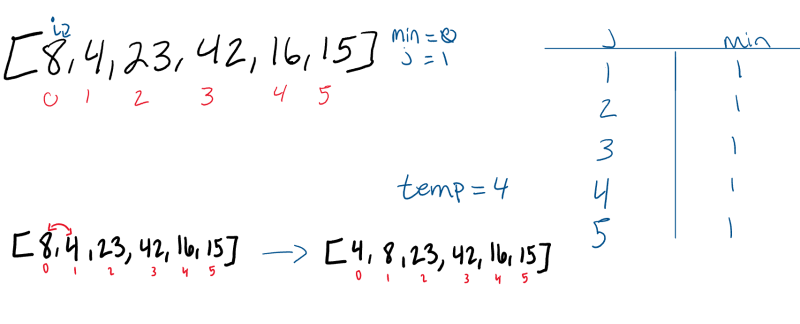
Our example below will be based on an array that looks like this at the start: [8,4,23,42,16,15]
Pass 1:
In the first pass-through of the selection sort, we evaluate if there is a smaller number in the array than what is currently present in index 0. This act is essentially finding the smallest number in the array and it will eventually place it in the very first index of the array. To do this, we must first evaluate what is placed in index 0 (in case the smallest value is already in the correct place) and check and see if a smaller number exists. We find this smaller number right away in index 1 (value of 4). The minimum variable gets updated to remember this index (j = 1), and the variable temp is updated with the index’s value (temp = 4). At the end of this iteration, after we verify there is no value smaller than 4, this number will be swapped with the current value (of 8) in index i (which is still 0). This results in our smallest number of our array being placed first.
Pass 2:
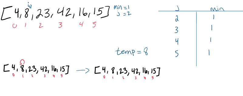
The second pass through the array evaluates the remaining values in the array to see if there is a smaller value other than the current position of i. 8 is the 2nd smallest number in the array, so it “swaps” with itself. The minimum value does not change at all during this “i = 1” iteration.
Pass 3:
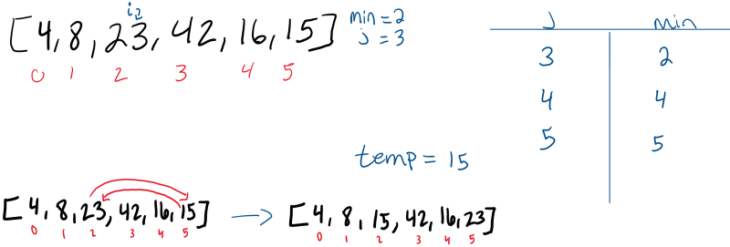
The third pass-through evaluates the remaining indexes in the array, starting at position “i = 2”. Both positions 4 and 5 are smaller than the value in position 2. Each time a smaller number than the current minimum is found, the min variable will update to the index of the new smallest number. In this case, 15 is the next smallest number. As a result, it will swap with the value in position 2.
Pass 4:
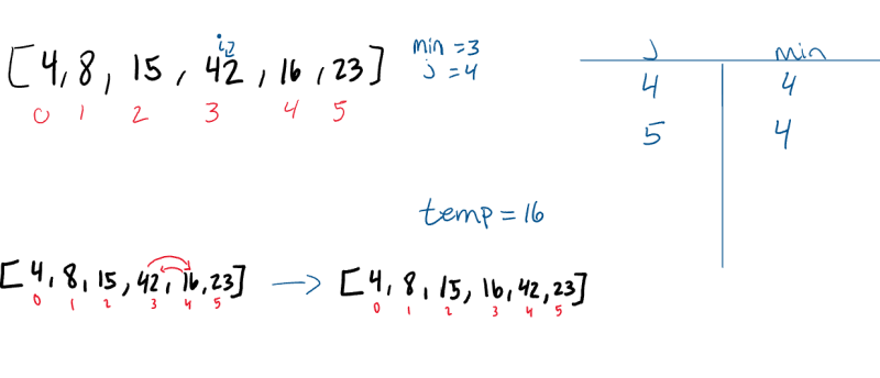
The 4th pass (i = 3) through the array finds that 16 is now the smallest number in the unsorted portion of the array, and as a result, switches places with the value 42.
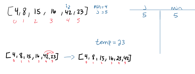
Pass 5:
The 5th pass (i = 4) through the array only has one other index to evaluate. Since the last index (j = 5) value is less than the value at the index of 4, the two values will swap.
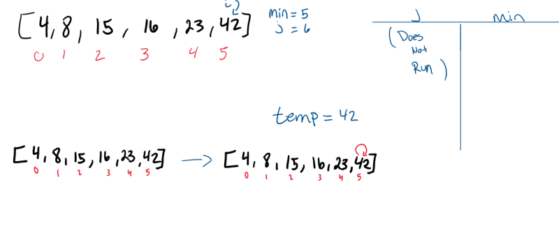
Pass 6:
On its final iteration through the array, it will swap places with itself as it evaluates the value against itself. After this iteration, i will increment to 6, forcing it to break out of the outer for loop, leaving our array sorted.
Can you see a way to modify the code to eliminate this step?
Complexity Analysis
Let’s evaluate the efficiency of this algorithm. As described here, the time complexity of selection sort is O(N^2). This is because for every index in the array, we must compare it against the remaining unsorted indexes to ensure that nothing “smaller” exists. The basic operation for selection sort can be thought of as a comparison operation. This comparison will occur an “n-squared” (divided by 2) number of times.
Selection Sort will usually be done in place, meaning that no extra memory or space needs to be created. As a result, we describe it as O(1) space complexity.
Summary
Amongst the world’s most popular sorting algorithms, selection sort is not the most efficient available, but it is straightforward to implement and is a great option when working with smaller data sets. As the data sets get larger, more efficient sorting algorithms shine. Many chose selection sort as a beginning sort to explore because of its simplicity and accessible implementation. Now that you have a baseline of comprehension, try coding it yourself in your favorite language, and see how this compares with other algorithms.